
SVM Doped
This is a simple image classifier for CIFAR-10 dataset. It is a Support Vector Machine (SVM) classifier with RBF kernel. It uses Principal Component Analysis (PCA) as dimensionality reduction and Histogram of Oriented Gradients (HOG) as feature extraction.
Introduction
In recent years, the use of machine learning has been increasing in many fields, including image classification. Nowadays, Deep Learning and Convolutional Neural Networks (CNN) are the most popular, if not default techniques for image classification. However, they are computationally expensive and require a lot of data.
In this project, I challenge myself to use “traditional” statistical models instead. One of the classics, Support Vector Machine (SVM) classifier, can be used to classify images. However, SVM alone does not provide good results. Therefore, I use Principal Component Analysis (PCA) as dimensionality reduction and Histogram of Oriented Gradients (HOG) as feature extraction to improve the performance of the classifier, as well as to reduce the computational cost and thus a faster training time.
Results
The results are not bad. The accuracy of the classifier is 0.62, with only 5 minutes of training time. That is not bad for a simple statistical model. In fact, when compared to students in my Machine Learning course, my result is of top 10%. The confusion matrix is shown below.

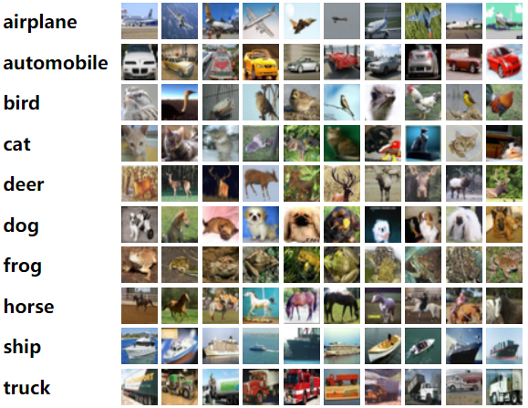
CIFAR-10 Dataset
The dataset consists of 60,000 32x32 color images in 10 different classes, with 6,000 images per class. There are 50,000 training images and 10,000 test images. The classes are completely mutually exclusive and there is no overlap between them.
Code
The code is available on Github. It is written in Python and Sklearn as a Jupyter Notebook. The code is developed on Google Colab. There is also I walkthrough video on YouTube.
Support Vector Machine
Support Vector Machine (SVM) is a supervised machine learning model that uses classification algorithms for two-group classification problems. SVM is a discriminative classifier formally defined by a separating hyperplane. In other words, given labeled training data (supervised learning), the algorithm outputs an optimal hyperplane which categorizes new examples.
Image below shows a linear SVM.

RBF Kernel
The RBF kernel is a popular kernel function used in various kernelized learning algorithms. It is a radial basis function (RBF), a function whose value depends only on the distance from the origin. The RBF kernel is a good default choice for many problems.
I have experimented with various kernels, including linear, polynomial, and sigmoid. RBF kernel gives the best result.
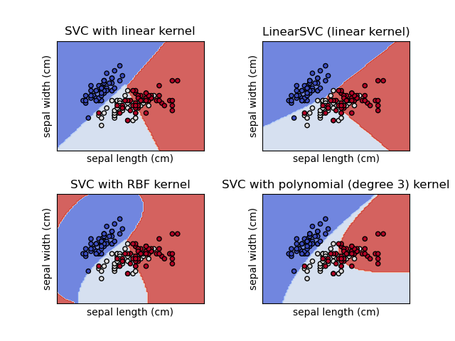
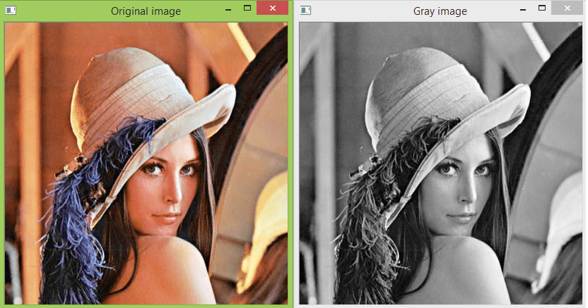
Image Grayscaling
The CIFAR-10 dataset consists of 32x32 color images. However, the 3 color channels added extra dimensionality which slows down the training process. Also, from the results of my experiments, colors do not provide better accuracy. Therefore, I convert the images to grayscale. This reduces the dimensionality of the data from 32x32x3 to 32x32.
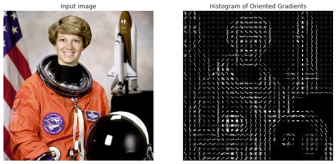
Feature Extraction via HOG
Histogram of Oriented Gradients (HOG) is a feature descriptor used in computer vision and image processing for the purpose of object detection. The technique counts occurrences of gradient orientation in localized portions of an image.
HOG alone boosted the accuracy of the classifier from 0.4 to 0.6. This makes sense because SVM alone is not really a classifier oriented towards images. The success of CNN is due to the fact that it is designed to work with images. It is designed to extract image related features like the edges, corners, and lines. HOG is doing similar things, but it is not as sophisticated as CNN. However, it is still a good and simple feature extractor for images.
Dimensionality Reduction Steps
- Input
32x32x3 => 3072 - Grayscaling
32x32x1 => 1024 - HOG
1024 => 324 - PCA
324 => 66
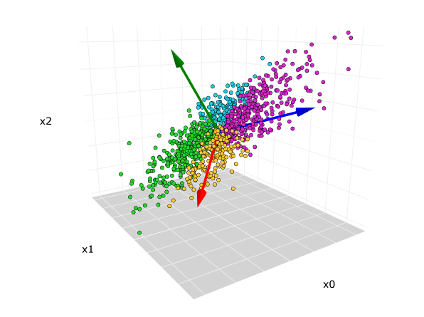
Dimensionality Reduction via PCA
Principal Component Analysis (PCA) is a statistical procedure that uses an orthogonal transformation to convert a set of observations of possibly correlated variables into a set of values of linearly uncorrelated variables called principal components. The first principal component accounts for as much of the variability in the data as possible, and each succeeding component in turn has the highest variance possible under the constraint that it is orthogonal to the preceding components.
In short, PCA finds in a multi-dimensional data, the few principal components that explain most of the variance in the data. It is a variance-maximising exercise.
From 324 features, to 66 features, with 80% of explained variance. This is a huge reduction in dimensionality. The accuracy of the classifier is not affected much, but the training time is reduced drastically.
PCA had helped reducing the training time drastically, from 1 hour to 5 minutes. Thanks to it, I was able to experiment with various parameters and models.
References
- CIFAR-10 Dataset
- Histogram of Oriented Gradients
- Principal Component Analysis
- Support Vector Machine
- RBF Kernel
- OpenCV
- Scikit-learn
- Google Colab
- Jupyter Notebook
Images
SVM Doped
This is a simple image classifier for CIFAR-10 dataset. It is a Support Vector Machine (SVM) classifier with RBF kernel. It uses Principal Component Analysis (PCA) as dimensionality reduction and Histogram of Oriented Gradients (HOG) as feature extraction.
Introduction
In recent years, the use of machine learning has been increasing in many fields, including image classification. Nowadays, Deep Learning and Convolutional Neural Networks (CNN) are the most popular, if not default techniques for image classification. However, they are computationally expensive and require a lot of data.
In this project, I challenge myself to use “traditional” statistical models instead. One of the classics, Support Vector Machine (SVM) classifier, can be used to classify images. However, SVM alone does not provide good results. Therefore, I use Principal Component Analysis (PCA) as dimensionality reduction and Histogram of Oriented Gradients (HOG) as feature extraction to improve the performance of the classifier, as well as to reduce the computational cost and thus a faster training time.
Results
The results are not bad. The accuracy of the classifier is 0.62, with only 5 minutes of training time. That is not bad for a simple statistical model. In fact, when compared to students in my Machine Learning course, my result is of top 10%. The confusion matrix is shown below.
CIFAR-10 Dataset
The dataset consists of 60,000 32x32 color images in 10 different classes, with 6,000 images per class. There are 50,000 training images and 10,000 test images. The classes are completely mutually exclusive and there is no overlap between them.
Code
The code is available on Github. It is written in Python and Sklearn as a Jupyter Notebook. The code is developed on Google Colab. There is also I walkthrough video on YouTube.
Support Vector Machine
Support Vector Machine (SVM) is a supervised machine learning model that uses classification algorithms for two-group classification problems. SVM is a discriminative classifier formally defined by a separating hyperplane. In other words, given labeled training data (supervised learning), the algorithm outputs an optimal hyperplane which categorizes new examples.
Image below shows a linear SVM.
RBF Kernel
The RBF kernel is a popular kernel function used in various kernelized learning algorithms. It is a radial basis function (RBF), a function whose value depends only on the distance from the origin. The RBF kernel is a good default choice for many problems.
I have experimented with various kernels, including linear, polynomial, and sigmoid. RBF kernel gives the best result.
Image Grayscaling
The CIFAR-10 dataset consists of 32x32 color images. However, the 3 color channels added extra dimensionality which slows down the training process. Also, from the results of my experiments, colors do not provide better accuracy. Therefore, I convert the images to grayscale. This reduces the dimensionality of the data from 32x32x3 to 32x32.
Feature Extraction via HOG
Histogram of Oriented Gradients (HOG) is a feature descriptor used in computer vision and image processing for the purpose of object detection. The technique counts occurrences of gradient orientation in localized portions of an image.
HOG alone boosted the accuracy of the classifier from 0.4 to 0.6. This makes sense because SVM alone is not really a classifier oriented towards images. The success of CNN is due to the fact that it is designed to work with images. It is designed to extract image related features like the edges, corners, and lines. HOG is doing similar things, but it is not as sophisticated as CNN. However, it is still a good and simple feature extractor for images.
Dimensionality Reduction Steps
- Input
32x32x3 => 3072 - Grayscaling
32x32x1 => 1024 - HOG
1024 => 324 - PCA
324 => 66
Dimensionality Reduction via PCA
Principal Component Analysis (PCA) is a statistical procedure that uses an orthogonal transformation to convert a set of observations of possibly correlated variables into a set of values of linearly uncorrelated variables called principal components. The first principal component accounts for as much of the variability in the data as possible, and each succeeding component in turn has the highest variance possible under the constraint that it is orthogonal to the preceding components.
In short, PCA finds in a multi-dimensional data, the few principal components that explain most of the variance in the data. It is a variance-maximising exercise.
From 324 features, to 66 features, with 80% of explained variance. This is a huge reduction in dimensionality. The accuracy of the classifier is not affected much, but the training time is reduced drastically.
PCA had helped reducing the training time drastically, from 1 hour to 5 minutes. Thanks to it, I was able to experiment with various parameters and models.
References
- CIFAR-10 Dataset
- Histogram of Oriented Gradients
- Principal Component Analysis
- Support Vector Machine
- RBF Kernel
- OpenCV
- Scikit-learn
- Google Colab
- Jupyter Notebook